Saturday, October 16, 2010

A walk down memory lane

I just found a page on "How to Find a Formula for a Set of Numbers".  It's a cool little procedure for taking a series, like:

2, 8, 9, 11, 20

and producing a polynomial to give you the next ones in the series, like:

n3- 17/2 n2+ 49/2 n - 15

where n is the term number, starting from n=1.  Try it out!  Anyway, it was a method I learned in high school math league, and thought it was so cool I wrote a BASIC program on the old TRS-80 computers to do it.  I had forgotten how to do it, and it was fun to see it again.  I particularly liked the comment on the page:

"""If someone gives you the sequence, say, "1, 4, 9, 16", you could run them through the above process and get the answer that the person is probably looking for: the rule is n2 so the next value is 25. But you could also invent any number as the next number in the sequence, say 42, and come up with a rule for "1, 4, 9, 16, 42". Feel free to work it out. It comes out to:


17/24 n4 - 85/12 n3 + 619/24 n2 - 425/12 n + 17
and the next term is then 121.

So if you want to be obnoxious, the next time you are given a quiz of "find the next number in the series" problems, just pick any number you like and fill it in, and you'll be completely correct. You'll probably get a failing grade on the test, but you can enjoy the smug satisfaction of knowing you were right."""

I knew a kid who, because of a ridiculous fluke, had to redo some of his middle-school competency tests in high school.  So, when presented with a series like 2,4,6,8,... he did this on a test (and yes he did fail the test and have to redo it).  He was also shown a number of clocks, and asked what time does this show, and for all of the answers put "analog time".

Friday, October 8, 2010

Power UnBalance

I love watching infomercials, but always wonder how much the sellers are exaggerating.  Take this infomercial for the "Power Balance" bracelet, which is claimed to increase balance and coordination:

http://www.youtube.com/watch?v=A_Ow-ZGMy5o

Now, go to this link which shows you how it actually works:

http://www.youtube.com/watch?v=Piu75P8sxTo

Make sure to watch the whole thing, because they give away the "trick" near the middle.  It is useful to go back afterward and watch the first one, now that you know the trick.

The real question, then, is: what should you do if you know a friend is considering buying this, or worse, has already bought it?  When I showed these videos in my class, I was told that the football team had purchased them already.  When some of my students presented them with the evidence, their response was that they didn't care whether it worked or not.

Astounding!

Saturday, September 25, 2010

Multiple Model Comparisons Revisited

Introduction

In a previous post, I hinted at how to do multiple hypotheses testing, using the ψ-measure. It turns out to be much clearer just using the posterior probabilities. The ψ-measure has a nice intuitive feel for the two-hypothesis case, but becomes convoluted in the multiple hyptheses case. Further, when introducing the application of Bayes theorem for students, I have found it to be clearer to follow the following procedure. We first look at Bayes theorem directly, for N hypotheses:

NewImage.jpg

We then calculate the numerator only, for every possible hypothesis:


NewImage.jpg


calculate the sum of all of these values,

NewImage.jpg

and then normalize

NewImage.jpg

The Octopus, Again


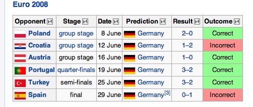
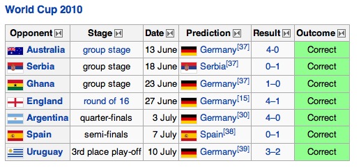
From the Wikipedia article, we have the following data:, which gave us correct=12 out of N=14:

  NewImage.jpg

NewImage.jpg

NewImage.jpg

The hypotheses that we consider are the following:

H = “Octopus is psychic, and can predict future (sports) events with 90% accuracy” R = “Octopus makes random choices” Y = “chooses flags with big yellow stripes 90% of the time” G = “chooses Germany 90% of the time”

Notice that both models Y and G, give us correct=12 for N=14 (if the “choosing Germany” chooses Spain in the Netherlands match, because of the similarity). The prior for the psychic octopus is, again, the very generous p(H) = 1/100. The two other non-random models should be more likely, before any data, so I take them to be p(Y)=p(G)=1/20. The random model, being the most likely, has the rest of the prior probability, p(R)=0.89.

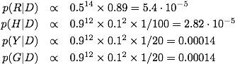
Now we calculate the numerators:

NewImage.jpg

Sum the values,

NewImage.jpg

and divide. achieving

NewImage.jpg

Thus, the two flag models went from being rare compared to random to being much more likely than random, and certainly much more likely than psychic. Bayes theorem, properly applied, is a quantitative embodiment of Carl Sagan’s famous quote “extraordinary claims require extraordinary evidence”. It is not just that the evidence must be extraordinary (like 999 correct out of 1000), but the evidence must be extraordinary to address all of the, somewhat rare but possible, hypotheses that would come up as much more likely given the initial result. The process of science is to perform experiments to address these alternative hypotheses.

Sunday, September 12, 2010

God and Hawking

From the book “The Grand Design” By STEPHEN HAWKING And LEONARD MLODINOW

....
Newton believed that our strangely habitable solar system did not "arise out of chaos by the mere laws of nature." Instead, he maintained that the order in the universe was "created by God at first and conserved by him to this Day in the same state and condition."

....

The press is pitching this book as a denial of God, claiming that Hawking has said that God does not exist. The media never seem to get the nuances of logical thinking, and its consequences.

What Hawking and Mlodinow are doing is a modernization of an approach used by Laplace (1749-1827) (http://en.wikipedia.org/wiki/Pierre-Simon_Laplace).  He worked on many things, including the dynamics of the solar system.  When Newton (http://en.wikipedia.org/wiki/Isaac_Newton) published his laws of dynamics 100 years earlier, he demonstrated that the speeds of the planets could be derived from a simple law of gravity.  In this way, Newton connected the Earthly things with the "Heavenly" things.  However, it was unclear to Newton whether the orbits of the planets would remain constant (as his religious philosophy would state), or if they would be unstable, change, and possibly fly apart given enough time.  He posited that one of the roles of God would be to nudge the planets, here and there, to keep their orbits stable.

Laplace, performing his calculations more precisely than his predecessors, was able to determine that the orbits would in fact be stable, without any extra tinkering.  Napoleon, when presented with the work of Laplace, asked him: "M. Laplace, they tell me you have written this large book on the system of the universe, and have never even mentioned its Creator."  Laplace replied, "I had no need of that hypothesis."

He did not say that there was no God (although that is what he believed), but that the concept of God was not necessary to explain the things that he was explaining using physics.  This included the formation of the solar system from a compressing ball of gas (due to gravity), which then forms the Sun in the center and the planets orbiting around.  This is essentially the model still in use today!

What Hawking is doing is basically the same thing, but with the origin of the universe.  Essentially the current model allows for the possibility of many universes to simultaneously exist and that, like a lottery winner, our universe supports life.  It may seem that the universe is "fine-tuned" to support human life, and that this would support the notion of an intelligent designer, Hawking is making the argument that a designer is not needed with our current understanding.  Like a lottery winner stating that the odds of winning are astronomical, and yet they won, and then reasoning that there was some design in this choice even when there wasn't.  As long as you have enough people playing (or enough universes) you'll eventually observe the unlikely, and that unlikely winner will feel singled out.  Hawking argues that the lottery winner (the life on Earth), is arguing the same way when it invokes a designer when it doesn't need to.  Hawking doesn't state "God doesn't exist", because that statement cannot be proven, but he simply states that it is an unnecessary hypothesis for the understanding of the origin of the universe.

Of course, *specific* Gods can be disproven.  For example, it is clear from many lines of evidence that the Earth is more the 6000 years old and that there never was a global flood.  However, you cannot disprove the notion of a God that creates the universe and is then hands-off, like deists commonly believe.  It is completely untestable.  It is also unnecessary, according to Hawking.  This doesn't make it wrong, it is just unnecessary in the same way that we don't need to invoke the divine when understanding how an apple falls from a tree.

Wednesday, September 1, 2010

Why pseudoscientists like the chi-square test (and why it shouldn't be taught)

In a prior post I outlined how orthodox statistics can lead to the either-or logical fallacies common in pseudoscience, like astrology and ufo-ology.

In this post I focus on the &chi2 test, it's pathologies, and why it is so useful for a pseudoscientist. The example is lifted from E. T. Jaynes' book "Probability Theory"

The two problems with &chi2 are:

  1. it violates your strong intuition in some simple cases
  2. it can lead to different results with the exact same data, binned in a different way


Both of these properties are useful to the pseudoscientist.

Intuition and Chi-square: The Three-sided coin


In each of this case we will have some data, and two models to compare which try to explain the data. Intuition strongly favors one, and &chi2 favors the other. One of my favorite problems is the three-sided coin: where the coin can fall heads, tails, or on the edge. Imagine we have two models for a relatively thick coin:


  • Model A: pheads=ptails=0.499, pedge=0.002
  • Model B: pheads=ptails=pedge=1/3


And we have the following data:


  • N=29: nheads=14, ntails=14, nedge=1


Which model are you more confident in? Model A of course! If we use the &psi-measure for goodness of fit with these two models, as defined in my prior post, then we have (remember: smaller &psi means more confident in the fit, just like smaller &chi2):


E7E94805-9E10-451E-9B95-C8EB2BA875C7.jpg


7AFD29D5-C801-416E-82AC-F9B363147B22.jpg


with &psiB-&psiA=26.85 which makes model A more then 100 times more likely than model B (a &psi difference of 20 would be exactly 100 times). Perfectly reasonable. What about &chi2?


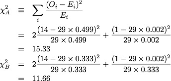
31844A12-1F3E-4D51-B2D0-EFAE00BE66A7.jpg


which makes model B slightly preferable to model A! Amazing! Where is this coming from? Apparently it is coming from the somewhat rare event of an edge-landing. If our data had been instead

  • N=29: nheads=15, ntails=14, nedge=0

then we'd have


  • &psiA=0.3
  • &psiB=51.2

and

  • &chi2A=0.093
  • &chi2B=14.55

where now both measures agree that model A is superior.


Why do pseudoscientists love the &chi2 test?
Answer 1: Because all they need to do is wait for that inevitable, somewhat rare but still possible, data point and &chi2 yields a pathologically high value


The &psi-measure and log-likelihood


To understand the other problem with the &chi2 test we need to understand what the &psi-measure is doing. As above, imagine we have a set of observations Oi. We define the total number of observed points and the relative frequency of each observation,


23229268-8820-42F8-BF8C-C984679DCB51.jpg


The maximum likelihood solution for the probabilities of observing Oi for each class, i, is just the relative frequency of each observation. This is the "just-so" solution, where we estimate the probability of seeing 14 heads in 29 flips as p=14/29. This "just-so" solution will have the closest match, and the highest likelihood (by definition). If we have a model which specifies a different set of probabilities for each class, then it's likelihood is simply


71272C22-E8B6-4497-82DF-FBDD89729630.jpg


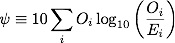
The &psi measure can be rewritten as


B363F3D7-1964-421A-A8E2-B19020D0117A.jpg


So you can think of the &psi-measure as comparing a model with the "just-so" solution (which has maximum likelihood). Further, subtracting one value of &psi with another (for different models) performs the log-likelihood ratio between the models. A proper analysis should include prior information, which can be done almost as easily.

An almost equivalent problem


Imagine that we have a coin with 6 faces, and we are comparing the following models:


  • Model A: p = [0.499/2, 0.499/2, 0.499/2, 0.499/2, 0.002/2,0.002/2]
  • Model B: p = [1/6,1/6,1/6,1/6,1/6,1/6]


And we have the following data:


  • N=29: O=[7,7,7,7,0,1]


where I have listed the probabilities and the outcomes for each face. Notice that, grouping them together in pairs we retrieve the same as the first example. Thus when comparing the two models, with this equivalent problem, we should get the same value. Because the size of the problem changed, the individual &psi values will be different (larger) because there are more terms in the "just-so" solution. However, the difference between the models should be the same. The results are:


  • &psiA=11.35 (old value 8.34)
  • &psiB=38.2 (old value 35.19)

with &psiB-&psiA=26.85 (old value 26.85...the same!), and

  • &chi2A=32.6 (old value 15.33)
  • &chi2B=11.76 (old value 11.66)


The &chi2 for one of the models (Model A) has been inflated quite a lot relative to the other model. This means that, depending on how you bin the data, you can make whichever model that you are looking at more or less significantly different, without changing the data at all.


Why do pseudoscientists love the &chi2 test?
Answer 2: Because all they need to do is bin their data in different ways to affect the level of significance of their model over the model to which they are comparing


Still taught?


So, why is the &chi2 test still taught? I don't know. It has pathological behavior in simple systems, where somewhat rare events artificially inflate its value, and it can be easily used to prop up an unreasonable model simply by rearranging the data. Why not teach something, like the &psi-measure, which is grounded theoretically in the likelihood principle and does not have such pathological behavior? If you prefer to use the log-likelihood instead, then that would be fine (and equivalent).

I think it is about time to purge the &chi2 test from our textbooks, and replace it with something correct.

Tuesday, August 31, 2010

Orthodox Statistics Conducive to Pseudo-Science

I have just realized that the thought process used in orthodox statistics is conducive to pseudo-science. It adds, in my opinion, to the long list of reasons why Bayesian inference is demonstrably superior (also see here). Let me show with a couple of simple examples.

Astrology

From this skeptical analysis of some astrology data, listing the numbers of famous rich people in each sign, we see the use of the chi-squared goodness of fit test. The data are:

SignNumber of People
Aries 95
Taurus 104
Gemini 110
Cancer 80
Leo 84
Virgo 88
Libra 87
Scorpio 79
Sagittarius 84
Capricorn 92
Aquarius 91
Pisces 73
Total 1067


To apply the chi-squared test, we simply compare the above numbers to the expected numbers if completely random, which is 1067 people/12=88.9 people according to:

7660DA25-CEEC-4B31-A199-76CEA69E5015.jpg


where O are the observed data and E are the expected counts. Once we have the chi-square value and the degrees of freedom (11 in this case), we can look up in tables to get the p-value:


5785E00F-983A-4B86-AF40-5F141440DD5A.jpg


Normally, this might be the end of the story, given that there is not even close to a significant value (usual cut-off around p=0.05).

Subset of the Data


So, if we only take the extreme values, say:

SignNumber of People
Gemini 110
Pisces 73
Total 183


then we calculate a different chi-squared, with 1 degree of freedom, and get


83387956-03D9-4DB0-810E-4BD2E7D836F1.jpg


Now this is pretty silly: of course, if you take the extreme values of 12 numbers, and pretend that they came from a 2-category situation, then it'll appear more significant. What about lumping 6 points together, say Capricorn to Gemini (the first part of the year) and the second part. In this case we aren't cherry picking, and the sums should be less significant than the individual data. We then have:

SignNumber of People
Capricorn-Gemini 565
Cancer-Sagittarius 502
Total 1067


And we expect 533.5 people in each category. Notice that we went from (the most extreme) 20 person difference from expected in about 100 to a 30 person difference in 500...closer to the expected. What do we get from our chi-squared test?


D9E69A77-09CD-43A1-88CF-256EB300D492.jpg


The test says that this is significantly different from random, more than the individual data! At least the goodness of fit measure, chi-squared value, went down to denote a closer fit to expected but the reduction in the number of data points changes the test quite a lot.

A different measure


E.T. Jaynes suggests in his book to use a different measure of goodness of fit, the &psi measure closely related to the log-likelihood


A210014E-5B3B-4DB4-AE14-63D0EB367E3D.jpg


Using this measure on the above examples, we get

  • All data: &psi = 28.9
  • Extreme data: &psi = 39.1
  • Lumped data: &psi = 8.1
which is completely in agreement with our intuition. The chi-squared test does not match our intuition, and seems to give significance to things that we know shouldn't be. But what about the test with the &psi-measure? How can we tell whether it is a significant difference? One could, in theory, give an arbitrary threshold but that would not be particularly useful, and would not be what a Bayesian would do. What a Bayesian would do is compare values of the goodness-of-fit measure to different models on the same data. It makes no sense, if you have only one model, to reject it by a statistical test...reject it in favor of what? If you have only one model, say Newton's Laws, and you have data that are extremely unlikely given that model, say the odd orbit of Mercury, you don't simply reject Newton's Laws until you have something else to put on the table. The either-or thinking of orthodox statistical tests is very similar to the either-or thinking of the pseudoscientist: either it is random, or it is due to some spiritual, metaphysical, astrological effect. You reject random, and thus you are forced to accept the only alternative put forward. I am not implying that all statisticians are supportive of pseudo-science, and they are often the first to say that you can only reject hypotheses not confirm them. However, since the method of using statistical tests does not stress the searching for alternatives, or better, the necessity for alternatives, it is conducive to these kinds of either-or logical fallacies. An example of a model comparison, from a Bayesian perspective, on a problem suffering from either-or fallacies can be found in the non-psychic octopus post I did earlier.

Friday, August 27, 2010

The Non-Psychic Octopus

Introduction


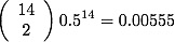
I saw in the newspaper an article about a supposedly psychic octopus, which predicts world cup matches by making a choice between two different foods labeled by the team flags. Paul the Octopus has an impressive record of 12 correct out of 14. Or is it impressive? How can we determine whether this performance is evidence for psychic behavior, or something else. A typical statistical analysis might start with the null hypothesis that the octopus was random, so was choosing the teams with probability p=0.5. The likelihood of getting 12 right in 14 is
217E3119-BC22-4A09-B534-D62BAA0BF53C.jpg


which is fantastically strong against the null! Even if you do the p-value test for the the correct data being more extreme, you get p-val=0.00646.

So, we reject the null, and the octopus must be psychic!...(or not)


Bayesian Analysis Against Random


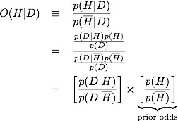
Let's look at this another way, and perhaps we can gain some insight. It will be convenient to talk about odds, rather then probability, and further to use the log of the odds so that this becomes an arithmetic problem. The odds is defined as the ratio of the probability for a hypothesis, H, and the probability for the inverse, not H.

E5899678-9897-42AF-8CBB-5D687A02A731.jpg


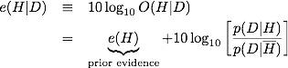
We define the log-odds, or evidence as defined by E. T. Jayes,

BAAC0566-3B79-4B44-8F0D-C5046788B491.jpg


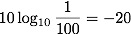
A few comments before we commence with more calculation. The prior evidence reflects our state of knowledge before we see the data. How likely is it that an octopus is psychic? Most reasonable people would say highly unlikely. Generous odds would be 100:1 against, although personally I'd probably put it at least a million to 1 against. Let's be generous. That gives us a prior evidence of

94E23FDD-36D3-4B6A-B72C-7C759FAAE1B1.jpg


If we had been naive, and set equal odds, then this evidence would be e=0. So we start with evidence e=-20 for a psychic octopus (which is strong evidence against it, because e<0), and then we observe the data. If we assume that a psychic octopus is right 90% of the time, and that the only alternative is a random octopus correct 50% of the time, then we have added evidence for each correct answer:


85F4C7A1-EFC7-4E8C-88B0-E98B846B1F97.jpg


Each incorrect answer gives:


D48A7B4A-112D-4BC6-A267-95B797A15F9C.jpg


The evidence gets pushed up from the prior with each correct answer, and down for each wrong answer. Notice how wrong answers are penalized more than right answers. This is because the psychic octopus is pretty good (p=0.9). We get a final (posterior) evidence for 12 correct and 2 wrong:


5BC4EE45-59BD-4A67-A2FF-779E7EC92145.jpg


which is about 2:1 odds against the psychic octopus.

More to the Story


Most pseudoscience gets propagated by people who reason naively. They will say that there are two possibilities, say random and psychic, and they they must both be equally likely before the data. So, when rare data is found, they reject random and claim this is evidence for psychic phenomena. This line of reasoning is incorrect for two reasons:

  1. random and psychic are not equally probable a priori - random is much more likely in cases like this
  2. there are more possibilities


We already saw how point (1) can be handled by proper prior information. Point (2), with multiple hypotheses gets mathematically a bit trickier (there are more terms to carry around) and is thus messier, but conceptually is fairly straightforward.

We have two hypotheses so far:

H="Octopus sees the correct future 90% of the time, and is psychic"


R="Octopus chooses randomly."


Let me introduce two more hypotheses.

Y="Octopus chooses flags with big yellow stripes 90% of the time"


G="Octopus chooses Germany 90% of the time"


How would you choose the prior probabilities for these hypotheses? Personally, as I said before, I'd have p(H) way below p(R) by about a factor of a million, but being generous, let's put it about a factor of 100. What about p(Y) and p(G)? I'd say that these might be comparable to random or, if I knew something about the vision of octopi or how the person feeding the octopus might rig the food in the direction of his favorite team, I might even have p(Y)>p(R) or p(G)>p(R). Certainly p(Y)>p(H) and p(G)>p(H). So what happens with the data?

For hypothesis Y, there are N=14 games of which the octopus chooses 12 with bright yellow stripes (there is one where it chose Germany over Ghana and should have chosen Ghana which has a bigger strips, and another with Germany and Spain where Spain should have been chosen). For hypothesis G there are N=14 games and the octopus chooses 12 for Germany (2 teams are chosen that are not Germany, and one match where Germany wasn't a choice and it chose Spain, which has the closest flag). Thus, the data support both of these hypotheses exactly as much as the p=0.9 psychic hypothesis. Therefore, the evidence will push these hypotheses up by as much as the psychic, over the random, and will make the psychic octopus even less likely.

So, when you hear fantastic claims supported with a comparison to random, the two things you must do are:

  1. Ask yourself what the prior probability of the fantastic claim is. Even if a random explanation is very rare, it will probably still be favored against the fantastic claim.
  2. Ask yourself what other possibilities, even if unlikely, could explain the data. Since the fantastic claim is exceedingly unlikely, even somewhat unlikely explanations may be supported by the data more than the original fantastic claim.